FinDeR Summer School (Part I): 3D point cloud alignment with optimal transport
What was the Frontiers in Design Representation Summer School (FinDeR)? Hosted by Prof. Mark Fuge at UMD College Park, it was a week long “summer school” where graduate students (including me) came together to learn and discuss how we represent design data for computation. The topics specific to this year’s summer school were optimal transport, information geometry, and generative models (e.g., VAEs, GANs). These topics were introduced in the context of how they may apply to data-driven design.
Motivation
I wanted to try techniques for working with 3D data since I know it is difficult to work with, yet much of design data is encoded into 3D objects such as CAD models or physical artifacts. One of the challenge problems was to try to match aorta scans between patients at different time points (younger and older) which seemed like a challenging but interesting task. Furthermore, this challenge did not have much data (only 8 .stl files) associated with it, allowing me to see how techniques might work in the face of limited data. I knew that it would not be possible to use what I had learned about generative models such as GANs with this amount of data. Furthermore, the techniques I learned from information geometry would be difficult to apply since they require knowing and being able to specify the manifold the data lies on. Thus, what I learned about optimal transport was a good option to try on this data.
Data
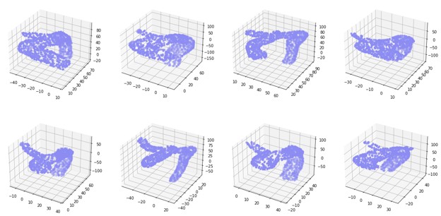
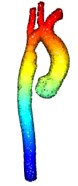
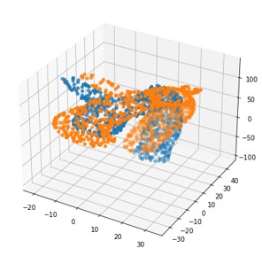
Each aorta was converted to a point cloud using the open3d library and 1000 points sampled from the .stl file. Initially, I did not apply any preprocessing to the point clouds. However, as I worked on the problem, I determined that certain preprocessing methods such as global registration could probably improve the results. My teammates and I realized (at the very end) that we likely needed to apply scaling as well.
Optimal Transport
This concept was introduced to us by Dr. Jean Feydy in the context of ways to transform points from source to target. More broadly, optimal transport is essentially a generalization of sorting to dimensions that are greater than one. It can be used, for example, to find the distance between unordered point clouds where you do not know the mapping between the points. To implement this idea in the context of the aorta 3D scans, I used the tutorial notebook provided by Dr. Feydy (available at here under Talks: Frontiers in Design Representation, University of Maryland) that demonstrated optimal transport in 2D, and extended it to 3D. When applying the concept of optimal transport, the loss was defined as follows:
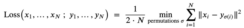
Notably, the Wasserstein distance is the square root of OT(A,B). Then, optimization needs to be performed to minimize this loss. This optimization can be conducted using gradient descent on the loss with respect to the features on the source object. In the tutorial, Dr. Feydy introduces the Sinkhorn algorithm, which I do not understand that well yet, within the optimization loop. Initially, I used the xyz-coordinates of the point cloud as the features (as an extension of the tutorial), despite knowing that it may not be the best representation for the structure of the aorta. The cost function in this case is the squared distance between the points of the two point clouds. Notably, optimal transport currently only works well for these types of simple cost functions since the pairwise costs between points have to be calculated.
Outcome
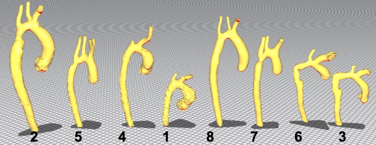
Since the 3D .stl files were available, a visual inspection could be performed to qualitatively assign each aorta to its respective pair, though the ground truth was initially unknown.
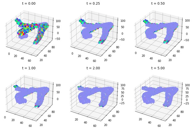
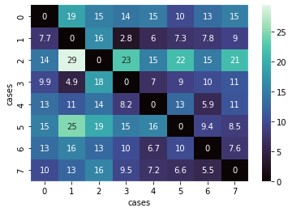
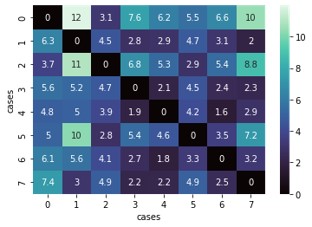
Then, the optimal transport loss was minimized over 100 time steps for each pair of aortas as the 1000-point point cloud as mentioned above. Below is a visualization of the optimal transport loss after 20 iterations. When the source and target were switched, the loss values were actually different (the optimization ended with a different permutation of points being mapped to each other). This is something I would have to investigate further to understand its impact on results.
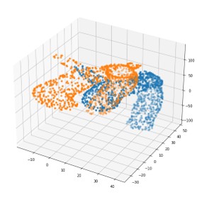
I then realized that some of the aortas were not aligned in 3D space, which is a problem for calculating a distance with xyz-coordinates as features. Dr. Feydy also noted that optimal transport does not generally work well if the distances are very large. To fix this issue, I decided to use open3d to perform global registration on the point clouds. This global registration is determined using fast point feature histograms, which are essentially features of each point based on its geometric neighbors. These features are matched to determine a transformation from source to target that aligns the point clouds.
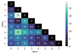
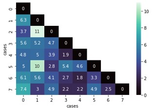
Again, the optimal transport loss was minimized and visualized, this time with the xyz-coordinates of the globally registered point clouds as features.
Finally, I attempted to address the issue of scaling by applying the iterative closest point (ICP) registration in open3d to get another transformation that includes scaling. The ICP algorithm requires an initial registration, which is satisfied by the transformation matrix obtained from global registration. However, this did not appear to make a difference in the optimal transport results.
Compared to our group’s qualitative assessment of which aortas looked like they would be paired, the results only corroborated one pair (7 & 8) without any registration and a different pair (3 & 6) after registration. However, the ground truth revealed at the end of the summer school was that the actual pairs were: 2 & 8, 1 & 4 (we assessed correctly), 3 & 6 (we assessed correctly), and 5 & 7. Looking back at the results, without global registration, only 5 & 7 could have been correctly paired using optimal transport. With global registration, 2 & 8, 3 & 6, and 5 & 7 could have been correctly paired. It was interesting how we were able to pair 1 & 4 visually while the optimal transport algorithm could not, yet it was able to pair 5 & 7 and 2 & 8 while we could not.
Lessons learned
Since the sizes of the aortas changed over the different scan times, the use of just xyz-coordinates is difficult: scaling matters. In addition, the xyz-coordinates do not capture geometric areas of the aorta that may vary across patients, but not over time. Using features that capture the general shape of the point cloud or domain-specific features (for example, the radius of specific arteries attached to the aorta) may have led to better outcomes. If there was more data, specifying the 3D features might become less important, as neural networks can be used to learn a latent representation of the object. Finally, although I learned about the concept of optimal transport, which is an interesting approach to compare two distributions, I would have to dig deeper into it to better understand its limitations compared to other approaches. Of course, both understanding and implementation is a huge barrier when trying to apply these types of advanced methods to complex problems, which is why I was limited to trying things that could be extended from existing implementations.